Detect water surface.

Most water bodies self level. Lidar elevation measurements of the water surface can frequently be detected by looking at histogram of the elevation measurements. The water surface will be flat except for any surface wave action, and even the waves can be accomodated with larger histogram bins. This function eaxmines the lidar elevatoin measurements and if it detects a flat surface which is above a threshold, it will return an object with attributes about the surface, including the detected water surface mean and median heights, and the standard deviation of those detected heights. It also returns a bool water_found.

import lidar_review_tools.lidar_tools as lt

source

detect_lidar_water_surface

 detect_lidar_water_surface (df, col='elev', thresh=4, binsize=0.1,
                             plot=True, height=4, width=10, title='Lidar
                             Water Surface Detector', xlabel='Elevations
                             [m]', ylabel='Range Bin Count',
                             title_fontsize=14, xlabel_fontsize=12,
                             ylabel_fontsize=12)

Find the water surface in a Pandas dataframe or numpy array.

	Type	Default	Details
df			DataFrame or Numpy data containing a column of LiDAR elevations.
col	str	elev	Label of elevation data.
thresh	int	4	Minimum number of elevations required for water surface detection.
binsize	float	0.1	Elevation binsize in meters.
plot	bool	True	Optionally generate plots of the elevation histogram, and inputelevations.
height	int	4	Height of the plot.
width	int	10	Width of the plot.
title	str	Lidar Water Surface Detector	Plot title.
xlabel	str	Elevations [m]	Plot X axis label.
ylabel	str	Range Bin Count	Plot Y axis label.
title_fontsize	int	14	Plot title font size, (points)
xlabel_fontsize	int	12	Plot xlabel font size, (points)
ylabel_fontsize	int	12	Plot ylabel font size (points)
Returns	object		A class containing attributes.

Testing

Colab

If you are testing this on Google Colab, run this cell to select the ATM data file for testing.

if __name__ == '__main__' and False:
  test_atm_fn = '/content/lidar_review_tools/data/atm/profile-1-atm-xyz.zip'
  ! head {test_atm_fn}

Docker Jlab.

Run this cell if you are running in the Docker Jlab

if __name__ == '__main__' and True:
  test_atm_fn = '~/work/github-projects/lidar_review_tools/data/atm/profile-1-atm-xyz.zip'

Now, let’s take a quicklook at the first 3 lines of the data in the file.
It is in classic CSV format. The first column is Longitude, second column is Latitude and the third is the elevation data.

! zcat {test_atm_fn} | head -3

-49.4788530000,69.0319020000,623.736
-49.4788610000,69.0318160000,624.403
-49.4788690000,69.0317280000,623.6

Load the ATM test data

Now load the test data into a Pandas DataFrameusing the Pandas read_csv() csv reader.
Since the data does not already have any column labels, we will add column names using the names parameter, and then via the read_csv() function.

if __name__ == '__main__' and True:
  atm = pd.read_csv(test_atm_fn, names=["lon", "lat", "elev"])

atm.head(3)

	lon	lat	elev
0	-49.478853	69.031902	623.736
1	-49.478861	69.031816	624.403
2	-49.478869	69.031728	623.600

plt.figure( figsize=(10,4))
plt.scatter( atm['lat'],  atm['elev'], marker='o', s=2 )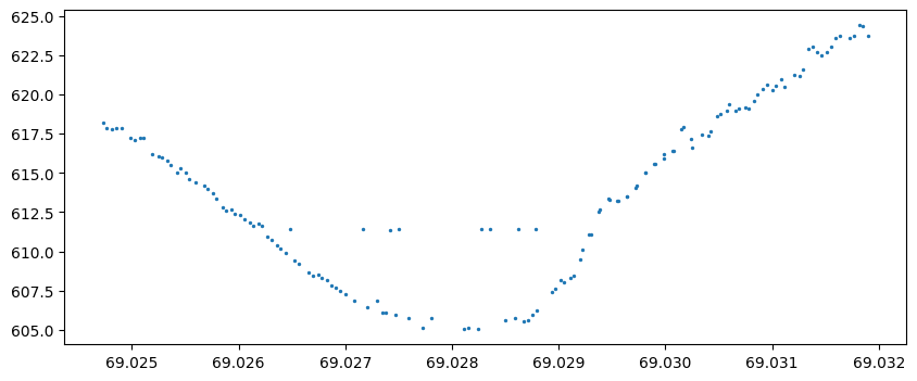

Load the ATM test profile dataset, run detect_lidar_water_surface() and plot the results.

## Test detect_lidar_water_surface()
if __name__ == '__main__' and True:
  rv = detect_lidar_water_surface(atm, plot=True, thresh=4, binsize = 0.1 )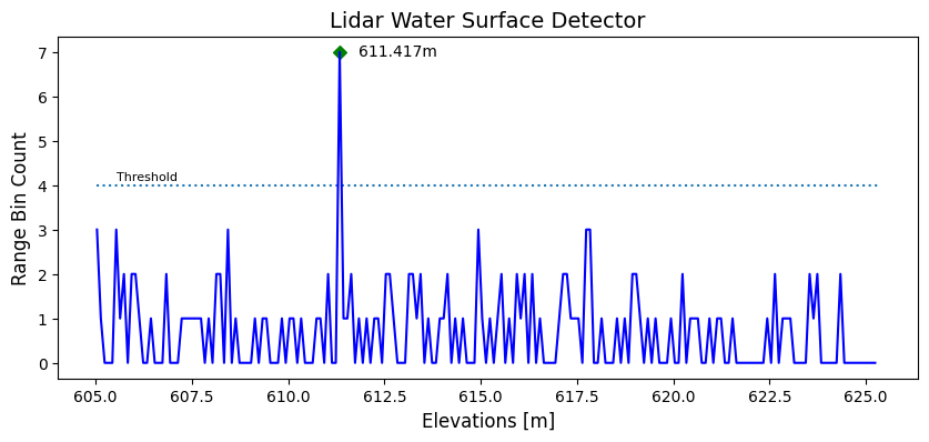

Printout the return `rv` data.

if __name__ == '__main__' and True:
  print("\nData returned by detect_lidar_water_surface()\n\n Key                 : Value\n-------------------------------")
  for i in rv.__dict__:
    if i == 'bins' or i == 'hist':
      continue
    if type( rv.__dict__[i] ) == np.float64:
      print(f"{i:20}: {rv.__dict__[i]:8.3f}")
    else:
      print(f'{i:20}: {rv.__dict__[i]}')


Data returned by detect_lidar_water_surface()

 Key                 : Value
-------------------------------
water_found         : True
binsize             : 0.1
thresh              : 4
plot                : True
ele_min             :  605.037
ele_max             :  624.403
surface_bin_value   :  611.337
peak_elevation_dif  :   19.366
max_v               : 7
surface_idx         : 63
low                 :  611.237
high                :  611.437
mean_surface        :  611.417
std_surface         :    0.015
median_surface      :  611.421

x = [atm['lat'].min(), atm['lat'].max()]
y = [rv.mean_surface,rv.mean_surface]
plt.figure( figsize=(10,4)) 
plt.plot( x, y, color='blue', alpha=.1)
plt.scatter(atm['lat'], atm['elev'], marker='o', s=2 )
plt.text( x[0], y[0]+.2, "Water Surface", fontsize=5)

Text(69.024727, 611.6167142857144, 'Water Surface')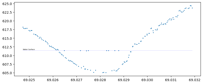

[69.024727, 69.031902]